Exponential distribution
Probability density function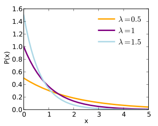 |
|
Cumulative distribution function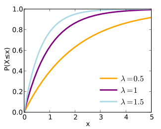 |
|
| parameters: |  rate or inverse scale (real) rate or inverse scale (real) |
|---|---|
| support: |  |
| pdf: |  |
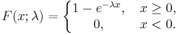
| cdf: |  |
| mean: |  |
| median: |  |
| mode: |  |
| variance: |  |
| skewness: |  |
| ex.kurtosis: |  |
| entropy: |  |
| mgf: |  |
| cf: |  |
In probability theory and statistics, the exponential distributions (a.k.a. negative exponential distributions) are a class of continuous probability distributions. They describe the times between events in a Poisson process, i.e. a process in which events occur continuously and independently at a constant average rate.
Contents |
Characterization
Probability density function
The probability density function (pdf) of an exponential distribution is
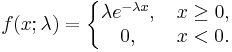
Here λ > 0 is the parameter of the distribution, often called the rate parameter. The distribution is supported on the interval [0, ∞). If a random variable X has this distribution, we write X ~ Exp(λ).
Cumulative distribution function
The cumulative distribution function is given by
Alternative parameterization
A commonly used alternative parameterization is to define the probability density function (pdf) of an exponential distribution as
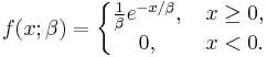
where β > 0 is a scale parameter of the distribution and is the reciprocal of the rate parameter, λ, defined above. In this specification, β is a survival parameter in the sense that if a random variable X is the duration of time that a given biological or mechanical system manages to survive and X ~ Exponential(β) then E[X] = β. That is to say, the expected duration of survival of the system is β units of time. The parameterisation involving the "rate" parameter arises in the context of events arriving at a rate λ, when the time between events (which might be modelled using an exponential distribution) has a mean of β = λ−1.
The alternative specification is sometimes more convenient than the one given above, and some authors will use it as a standard definition. This alternative specification is not used here. Unfortunately this gives rise to a notational ambiguity. In general, the reader must check which of these two specifications is being used if an author writes "X ~ Exponential(λ)", since either the notation in the previous (using λ) or the notation in this section (here, using β to avoid confusion) could be intended.
Occurrence and applications
The exponential distribution occurs naturally when describing the lengths of the inter-arrival times in a homogeneous Poisson process.
The exponential distribution may be viewed as a continuous counterpart of the geometric distribution, which describes the number of Bernoulli trials necessary for a discrete process to change state. In contrast, the exponential distribution describes the time for a continuous process to change state.
In real-world scenarios, the assumption of a constant rate (or probability per unit time) is rarely satisfied. For example, the rate of incoming phone calls differs according to the time of day. But if we focus on a time interval during which the rate is roughly constant, such as from 2 to 4 p.m. during work days, the exponential distribution can be used as a good approximate model for the time until the next phone call arrives. Similar caveats apply to the following examples which yield approximately exponentially distributed variables:
- The time until a radioactive particle decays, or the time between clicks of a geiger counter
- The time it takes before your next telephone call
- The time until default (on payment to company debt holders) in reduced form credit risk modeling
Exponential variables can also be used to model situations where certain events occur with a constant probability per unit length, such as the distance between mutations on a DNA strand, or between roadkills on a given road.
In queuing theory, the service times of agents in a system (e.g. how long it takes for a bank teller etc. to serve a customer) are often modeled as exponentially distributed variables. (The inter-arrival of customers for instance in a system is typically modeled by the Poisson distribution in most management science textbooks.) The length of a process that can be thought of as a sequence of several independent tasks is better modeled by a variable following the Erlang distribution (which is the distribution of the sum of several independent exponentially distributed variables).
Reliability theory and reliability engineering also make extensive use of the exponential distribution. Because of the memoryless property of this distribution, it is well-suited to model the constant hazard rate portion of the bathtub curve used in reliability theory. It is also very convenient because it is so easy to add failure rates in a reliability model. The exponential distribution is however not appropriate to model the overall lifetime of organisms or technical devices, because the "failure rates" here are not constant: more failures occur for very young and for very old systems.
In physics, if you observe a gas at a fixed temperature and pressure in a uniform gravitational field, the heights of the various molecules also follow an approximate exponential distribution. This is a consequence of the entropy property mentioned below.
Properties
Mean, variance, and median
The mean or expected value of an exponentially distributed random variable X with rate parameter λ is given by
![\mathrm{E}[X] = \frac{1}{\lambda}. \!](/I/a12c0f2b9a3efd768c970f0ddf6535d4.png)
In light of the examples given above, this makes sense: if you receive phone calls at an average rate of 2 per hour, then you can expect to wait half an hour for every call.
The variance of X is given by
![\mathrm{Var}[X] = \frac{1}{\lambda^2}. \!](/I/dab5a58e08e019e1b28a884a2caa19c2.png)
The median of X is given by
![\text{m}[X] = \frac{\ln 2}{\lambda} < \text{E}[X], \!](/I/ce2ceedcc65691cb0ec79b6940ee0ada.png)
where ln refers to the natural logarithm. Thus the absolute difference between the mean and median is
![| \text{E}[X]- \text{m}[X]| = \frac{1- \ln 2}{\lambda}< \frac{1}{\lambda} = \text{standard deviation},](/I/3e79242040e24a6751e47212a0ad7596.png)
in accordance with the median-mean inequality.
Memorylessness
An important property of the exponential distribution is that it is memoryless. This means that if a random variable T is exponentially distributed, its conditional probability obeys

This says that the conditional probability that we need to wait, for example, more than another 10 seconds before the first arrival, given that the first arrival has not yet happened after 30 seconds, is equal to the initial probability that we need to wait more than 10 seconds for the first arrival. So, if we waited for 30 seconds and the first arrival didn't happen (T > 30), probability that we'll need to wait another 10 seconds for the first arrival (T > 30 + 10) is the same as the initial probability that we need to wait more than 10 seconds for the first arrival (T > 10). This is often misunderstood by students taking courses on probability: the fact that Pr(T > 40 | T > 30) = Pr(T > 10) does not mean that the events T > 40 and T > 30 are independent.
To summarize: "memorylessness" of the probability distribution of the waiting time T until the first arrival means

It does not mean

(That would be independence. These two events are not independent.)
The exponential distributions and the geometric distributions are the only memoryless probability distributions.
The exponential distribution also has a constant hazard function.
Quartiles
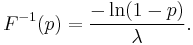
The quantile function (inverse cumulative distribution function) for Exponential(λ) is
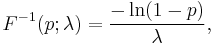
for 0 ≤ p < 1. The quartiles are therefore:
- first quartile

- median

- third quartile

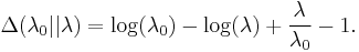
Kullback–Leibler divergence
The directed Kullback–Leibler divergence between Exp(λ0) ('true' distribution) and Exp(λ) ('approximating' distribution) is given by
Maximum entropy distribution
Among all continuous probability distributions with support [0,∞) and mean μ, the exponential distribution with λ = 1/μ has the largest entropy.
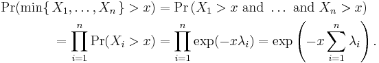
Distribution of the minimum of exponential random variables
Let X1, ..., Xn be independent exponentially distributed random variables with rate parameters λ1, ..., λn. Then
is also exponentially distributed, with parameter
This can be seen by considering the complementary cumulative distribution function:
The index of the variable which achieves the minimum is distributed according to the law
Note that
is not exponentially distributed.
Parameter estimation
Suppose a given variable is exponentially distributed and the rate parameter λ is to be estimated.
Maximum likelihood
The likelihood function for λ, given an independent and identically distributed sample x = (x1, ..., xn) drawn from the variable, is

where

is the sample mean.
The derivative of the likelihood function's logarithm is
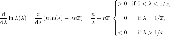
Consequently the maximum likelihood estimate for the rate parameter is

While this estimate is the most likely reconstruction of the true parameter  , it is only an estimate, and as such, one can imagine that the more data points are available the better the estimate will be. It so happens that one can compute an exact confidence interval – that is, a confidence interval that is valid for all number of samples, not just large ones. The 100(1 − α)% exact confidence interval for this estimate is given by[1]
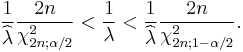
Where  is the MLE estimate, is the true value of the parameter, and
  is the value of the chi squared distribution with
  degrees of freedom that gives
  cumulative probability (i.e. the value found in chi-squared tables [1]).
Bayesian inference
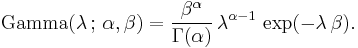
The conjugate prior for the exponential distribution is the gamma distribution (of which the exponential distribution is a special case). The following parameterization of the gamma pdf is useful:
The posterior distribution p can then be expressed in terms of the likelihood function defined above and a gamma prior:
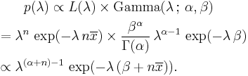
Now the posterior density p has been specified up to a missing normalizing constant. Since it has the form of a gamma pdf, this can easily be filled in, and one obtains

Here the parameter α can be interpreted as the number of prior observations, and β as the sum of the prior observations.
Prediction
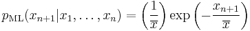
Having observed a sample of  data points from an unknown exponential distribution a common task is to use these samples to make predictions about future data from the same source. A common predictive distribution over future samples is the so-called plug-in distribution, formed by plugging a suitable estimate for the rate parameter into the exponential density function. A common choice of estimate is the one provided by the principle of maximum likelihood, and using this yields the predictive density over a future sample xn+1, conditioned on the observed samples x = (x1, ..., xn) given by
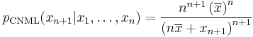
The Bayesian approach provides a predictive distribution which takes into account the uncertainty of the estimated parameter, although this may depend crucially on the choice of prior. A recent alternative that is free of the issues of choosing priors is the Conditional Normalized Maximum Likelihood (CNML) predictive distribution [2]
The accuracy of a predictive distribution may be measured using the distance or divergence between the true exponential distribution with rate parameter,  , and the predictive distribution based on the sample x. The Kullback–Leibler divergence is a commonly used, parameterisation free measure of the difference between two distributions. Letting
  denote the Kullback–Leibler divergence between an exponential with rate parameter and a predictive distribution
  it can be shown that
![\begin{align}
{\rm E}_{\lambda_0} \left[ \Delta(\lambda_0||p_{\rm ML}) \right] &= \psi(n) + \frac{1}{n-1} - \log n \\
{\rm E}_{\lambda_0} \left[ \Delta(\lambda_0||p_{\rm CNML}) \right] &= \psi(n) + \frac{1}{n} - \log n \\
\end{align}](/I/99200d2cc41d091b5ac3cefe9c9ce760.png)
where the expectation is taken with respect to the exponential distribution with rate parameter  , and
, and  is the digamma function. It is clear that the CNML predictive distribution is strictly superior to the maximum likelihood plug-in distribution in terms of average Kullback–Leibler divergence for all sample sizes
  .
.
Generating exponential variates
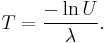
A conceptually very simple method for generating exponential variates is based on inverse transform sampling: Given a random variate U drawn from the uniform distribution on the unit interval (0, 1), the variate
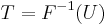
has an exponential distribution, where F −1 is the quantile function, defined by
Moreover, if U is uniform on (0, 1), then so is 1 − U. This means one can generate exponential variates as follows:
Other methods for generating exponential variates are discussed by Knuth[3] and Devroye.[4]
The ziggurat algorithm is a fast method for generating exponential variates.
A fast method for generating a set of ready-ordered exponential variates without using a sorting routine is also available.[4]
Related distributions
- An exponential distribution is a special case of a gamma distribution with
 (or
(or  depending on the parameter set used).
 - Both an exponential distribution and a gamma distribution are special cases of the phase-type distribution.
 , i.e. Y has a Weibull distribution, if
  and
and  . In particular, every exponential distribution is also a Weibull distribution.
 , i.e. Y has a Rayleigh distribution, if
 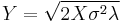 and
and  .
. , i.e. Y has a Gumbel distribution if
 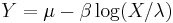 and .
and . , i.e. Y has a Laplace distribution, if
  for two independent exponential distributions
  and
and  .
. , i.e. Y has an exponential distribution if
  for independent exponential distributions
  .
. , i.e. Y has a uniform distribution if
  and .
and . , i.e. X has a chi-square distribution with 2 degrees of freedom, if
  .
.- Let
 be exponentially distributed and independent and
  . Then
  , i.e. Y has a Gamma distribution.
  , then
  : see skew-logistic distribution.
- Let
 and
and  be independent. Then
  has probability density function
 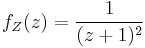 . This can be used to obtain a confidence interval for
  .
.
Other related distributions:
- Hyper-exponential distribution – the distribution whose density is a weighted sum of exponential densities.
- Hypoexponential distribution – the distribution of a general sum of exponential random variables.
- exGaussian distribution – the sum of an exponential distribution and a normal distribution.
See also
- Dead time – an application of exponential distribution to particle detector analysis.
References
- ↑ K. S. Trivedi, Probability and Statistics with Reliability, Queueing and Computer Science applications, Chapter 10 Statistical Inference, http://www.ee.duke.edu/~kst/BLUEppt/chap10f_secure.pdf
- ↑ D. F. Schmidt and E. Makalic, "Universal Models for the Exponential Distribution", IEEE Transactions on Information Theory, Volume 55, Number 7, pp. 3087–3090, 2009 doi:10.1109/TIT.2009.2018331
- ↑ Donald E. Knuth (1998). The Art of Computer Programming, volume 2: Seminumerical Algorithms, 3rd edn. Boston: Addison–Wesley. ISBN 0-201-89684-2. See section 3.4.1, p. 133.
- ↑ 4.0 4.1 Luc Devroye (1986). Non-Uniform Random Variate Generation. New York: Springer-Verlag. ISBN 0-387-96305-7. See chapter IX, section 2, pp. 392–401.
|
||||||||||||||||||||||||||||||||||||||||||||||||||||||||||||||||||
|
|||||||||||